The Haar wavelet-based perceptual similarity index (HaarPSI) is a similarity measure for images that aims to correctly assess the perceptual similarity between two images with respect to a human viewer.
In most practical situations, images and videos can neither be compressed nor transmitted without introducing distortions that will eventually be perceived by a human observer. Vice versa, most applications of image and video restoration techniques, such as inpainting or denoising, aim to enhance the quality of experience of human viewers. Correctly predicting the similarity of an image with an undistorted reference image, as subjectively experienced by a human viewer, can thus lead to significant improvements in any transmission, compression, or restoration system.
The HaarPSI has the following advantages over previous full reference quality metrics such as (MS-)SSIM, FSIM, PSNR, GSM, or VIF:
It achieves higher correlations with human opinion scores on large benchmark databases in almost every case (see experimental results).
It can be computed very efficiently and significantly faster than most other metrics (see Table II in our paper).
Downloads
You can download MATLAB and Python functions implementing the HaarPSI here:
If you use the HaarPSI in your research, please cite the following paper:
R. Reisenhofer, S. Bosse, G. Kutyniok and T. Wiegand. A Haar Wavelet-Based Perceptual Similarity Index for Image Quality Assessment.(PDF)
Signal Processing: Image Communication, vol. 61, 33-43, 2018. doi:10.1016/j.image.2017.11.001
Usage
In MATLAB, the HaarPSI can be computed by passing two images of the same size to HaarPSI.m.
HaarPSI.m accepts both RGB and grayscale images as input. Please make sure that the values are given in the \([0,255]\) interval!
Please note that by default, both images are being preprocessed by the convolution with a \(2\times2\) mean filter as well as a subsequent dyadic subsampling step, to simulate the typical distance between an image and its viewer. To omit this preprocessing step, you can pass 0 as a third argument to HaarPSI, as shown in the example below.
The Haar Wavelet-Based Perceptual Similarity Index
The HaarPSI expresses the perceptual similarity of two digital images in the interval \([0,1]\), that is
$$\operatorname{HaarPSI}\colon \ell^2({\mathbb{Z}^2})\times\ell^2({\mathbb{Z}^2}) \rightarrow [0,1],$$
such that the HaarPSI of two identical images will be exactly one and the HaarPSI of two completely different images will be close to zero.
The first step in the computation of the HaarPSI is the construction of similarity maps based on local features obtained for both images.
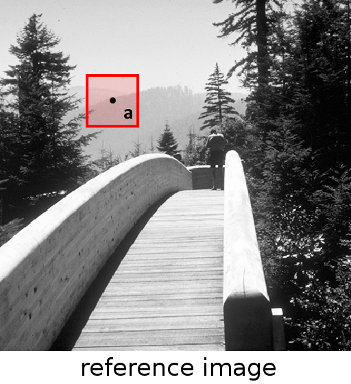
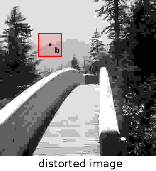
The HaarPSI of two images is based on the similarity of local features \(a\) and \(b\).
To assess the similarity of local features \(a, b \in \mathbb{R}\), a simple similarity measure for scalar values that already appeared in [2] is used:
$$
\operatorname{S}(a,b,C) = \frac{2ab + C}{a^2 + b^2 + C},
$$
with a constant \(C > 0\).
In the HaarPSI, the features of two grayscale images \(f_{1},f_{2}\in\ell^2(\mathbb{Z}^2)\) used to construct local similarity maps are based on the coefficients of a discrete wavelet transform. The wavelet chosen for HaarPSI is the so-called Haar wavelet, which was already proposed in 1910 by Alfred Haar [1] and is arguably the simplest and computationally most efficient wavelet there is. The one-dimensional Haar filters are given by
$$
h^{\text{1D}}_1 = \frac{1}{\sqrt{2}}\cdot[1,1] \text{ and } g^{\text{1D}}_1 = \frac{1}{\sqrt{2}}\cdot[-1,1],
$$
where \(h^{\text{1D}}_1\) denotes the low-pass scaling filter and \(g^{\text{1D}}_1\) the corresponding high-pass wavelet filter.
For any scale \(j\in\mathbb{N}\), we can construct two-dimensional Haar filters by setting
$$
\begin{align*}
g^{\text{(1)}}_j &= g^{\text{1D}}_j \otimes h^{\text{1D}}_j,\\
g^{\text{(2)}}_j &= h^{\text{1D}}_j \otimes g^{\text{1D}}_j,
\end{align*}
$$
where \(\otimes\) denotes the outer product and the one-dimensional filters \(h^{\text{1D}}_j\) and \(g^{\text{1D}}_j\) are given for \(j>1\) by
$$
\begin{align*}
g^{\text{1D}}_j &= h^{\text{1D}}_{1}*(g^{\text{1D}}_{j-1})_{\uparrow 2}, \\
h^{\text{1D}}_j &= h^{\text{1D}}_{1}*(h^{\text{1D}}_{j-1})_{\uparrow 2},
\end{align*}
$$
where \(\uparrow2\) is the dyadic upsampling operator, and \(*\) denotes the one-dimensional convolution operator. Note that \(g^{\text{(1)}}_j\) responds to horizontal structures, while \(g^{\text{(2)}}_j\) picks up vertical structures.
The six horizontal and vertical Haar wavelet filters used in the HaarPSI.
To correctly predict the perceptual similarity experienced by human viewers, it can be useful to apply an additional non-linear mapping to the local similarities obtained from high-frequency Haar wavelet filter responses. This non-linearity is chosen to be the logistic function, which is widely used as an activation function in neural networks for modeling thresholding in biological neurons and is given for a parameter \(\alpha >0\) as
$$
l_\alpha(x) = \frac{1}{1 + e^{-\alpha x}}.
$$
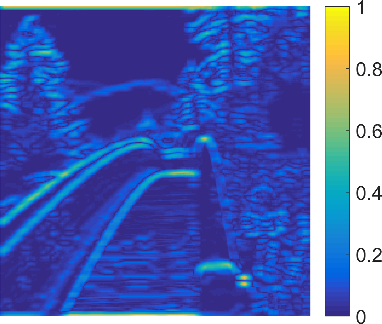
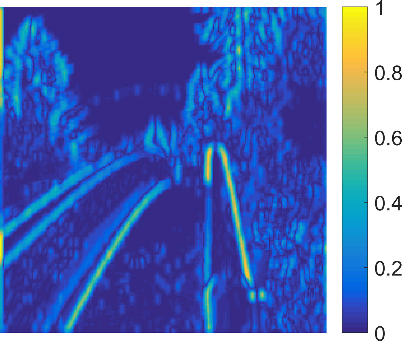
For two grayscale images \(f_1,f_2\in\ell^2(\mathbb{Z}^2)\), we define a local similarity measure based on the first two stages of a two-dimensional discrete Haar wavelet transform, namely
$$
\operatorname{HS^\text{(k)}_{f_1,f_2}}[x]=l_\alpha\left(\frac{1}{2}\sum_{j= 1}^2\operatorname{S}\left(\vert(g^\text{(k)}_j*f_1)[x]\vert,\vert(g^\text{(k)}_j*f_2)[x]\vert,C\right)\right),
$$
where \(C > 0\) is a constant, \(k\in\{1,2\}\) selects either horizontal or vertical filters, \(\operatorname{S}\) denotes the scalar similarity measure, and \(*\) is the two-dimensional convolution operator.
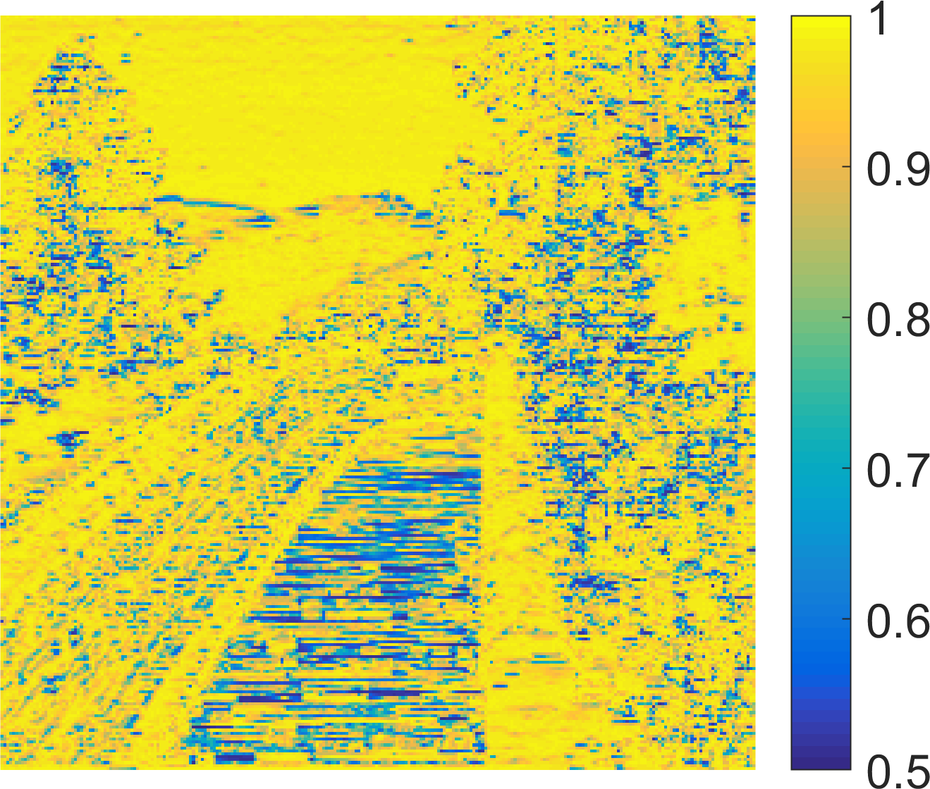
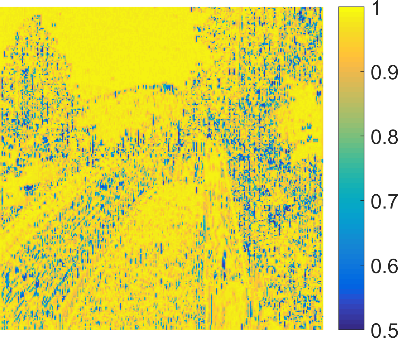
The local similarity maps \(\operatorname{HS^\text{(1)}_{f_1,f_2}}\) (left) and \(\operatorname{HS^\text{(2)}_{f_1,f_2}}\) (right).
To define a single similarity index for two images, all values from the previously defined similarity maps are combined by computing their weighted mean. The corresponding weights are based on the third scale of a discrete Haar wavelet transform and given by
$$
\operatorname{W^\text{(k)}_{f}}[x] = \left\vert(g^{\text{(k)}}_3*f)[x]\right\vert,
$$
where \(k\in\{1,2\}\) again differentiates between horizontal and vertical filters. Note that this weight function can be seen as an analog to phase congruency measure [10] used for a similar purpose in the definition of FSIM [3].
The weight functions \(\operatorname{W^\text{(1)}_{f}}\) (left) and \(\operatorname{W^\text{(2)}_{f}}\) (right).
The Haar wavelet-based perceptual similarity index for two grayscale images \(f_1,f_2\) is finally given by
$$
\operatorname{HaarPSI_{f_1,f_2}} = l_\alpha^{-1}\left(\frac{\sum\limits_x \sum\limits_{k=1}^2\operatorname{HS^\text{(k)}_{f_1,f_2}}[x] \cdot \operatorname{W^\text{(k)}_{f_1,f_2}}[x]}{\sum\limits_x \sum\limits_{k=1}^2\operatorname{W^\text{(k)}_{f_1,f_2}}[x]}\right)^2,
$$
with \(\operatorname{W^\text{(k)}_{f_1,f_2}}[x] = \max(\operatorname{W^\text{(k)}_{f_1}}[x],\operatorname{W^\text{(k)}_{f_2}}[x])\).
The HaarPSI can be extended to color images in the YIQ color space by including the chroma channels I and Q in the local similarity measure. This generalization is given by
$$
\operatorname{HaarPSIC_{f_1,f_2}} = l_\alpha^{-1}\left(\frac{\sum\limits_x \sum\limits_{k=1}^3\operatorname{HS^\text{(k)}_{f_1,f_2}}[x] \cdot \operatorname{W^\text{(k)}_{f^\text{Y}_1,f^\text{Y}_2}}[x]}{\sum\limits_x \sum\limits_{k=1}^3\operatorname{W^\text{(k)}_{f^\text{Y}_1,f^\text{Y}_2}}[x]}\right)^2,
$$
with \(\operatorname{HS^\text{(1)}_{f_1,f_2}}\) and \(\operatorname{HS^\text{(2)}_{f_1,f_2}}\) as in the definition of \(\operatorname{HaarPSI_{f_1,f_2}}\) and a chroma-sensitive local similarity measure
$$
\operatorname{HS^\text{(3)}_{f_1,f_2}}[x]=l_\alpha\left(\frac{1}{2}\left(\operatorname{S}\left(\vert(m*f^{\text{I}}_1)[x]\vert,\vert(m*f^{\text{I}}_2)[x]\vert,C\right) + \operatorname{S}(\vert(m*f^{\text{Q}}_1)[x]\vert,\vert(m*f^{\text{Q}}_2)[x]\vert,C)\right)\right)
$$
with a \(2\times2\) mean filter \(m\) and
$$
\operatorname{W^\text{(3)}_{f^\text{Y}_1,f^\text{Y}_2}}[x] = \frac{1}{2}\left(\operatorname{W^\text{(1)}_{f^\text{Y}_1,f^\text{Y}_2}}[x]+\operatorname{W^\text{(2)}_{f^\text{Y}_1,f^\text{Y}_2}}.[x]\right).
$$
The HaarPSI only requires two parameters to be selected, namely \(C\) and \(\alpha\). These parameters were optimized to yield a superior overall performance on all benchmark databases on which the HaarPSI was evaluated. The parameters were eventually chosen to be \(C = 30\), \(\alpha = 4.2\). It should be noted that for other databases or specific applications, different values might still be favorable (see for example Fig. 4 in our paper).
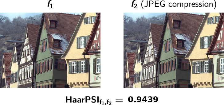
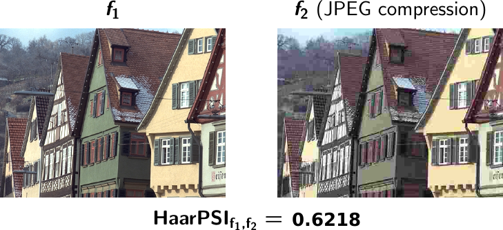
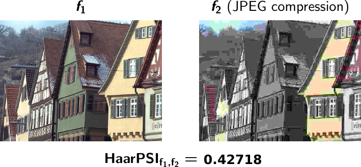
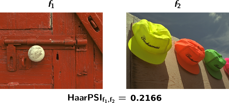
Examples of the HaarPSI for different pairs of images.
Experimental Results
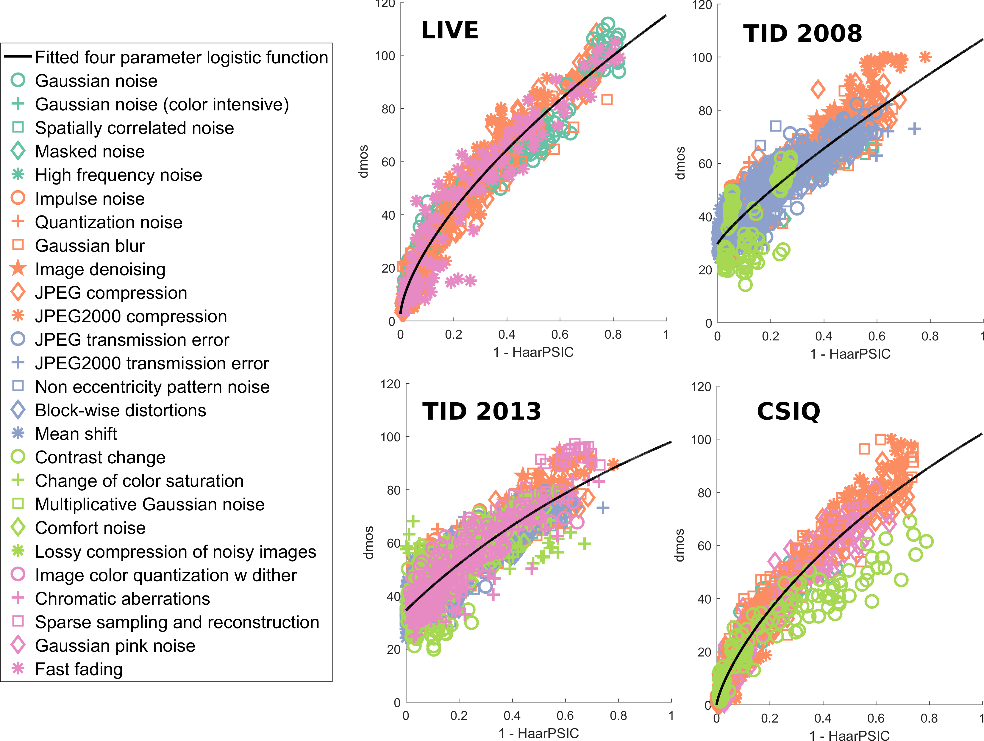
The consistency of HaarPSI with the human perception of image quality was evaluated and compared with most state-of-the-art image similarity measures via four large publicly available benchmark databases of quality-annotated images (LIVE [11], TID 2008 [12], TID 2013 [13] and CSIQ [5]).
The following tables depict the Spearman rank order correlation coefficients (SROCC) with the human opinion scores for all four databases and ten different image similarity measures. The highest correlation in each row is written in boldface.
Detailed tables reporting Spearman and Kendall rank order correlations as well as Pearson correlations before and after non-linear regression can be found here. These tables also include an analysis of statistical significance and distortion specific results for all four databases.
Scatter plots of HaarPSIC values against difference mean opinions scores (DMOS) from the LIVE, TID 2008, TID 2013 and CSIQ image databases.
References
A. Haar, Zur Theorie der orthogonalen Funktionensysteme, Mathematische Annalen, vol. 69, no. 3, pp. 331-371, 1910.
Z. Wang, A. C. Bovik, H. R. Sheikh, and E. P. Simoncelli, Image quality assessment: From error visibility to structural similarity, IEEE Trans. Image Proc., vol. 13(4), pp. 600-612, 2004.
L. Zhang, L. Zhang, X. Mou, and D. Zhang, Fsim: A feature similarity index for image quality assessment, IEEE Trans. Image Proc., vol. 20(8), pp. 2378-2386, 2011.
L. Zhang, Y. Shen, and H. Li, Vsi: A visual saliency-induced index for perceptual image quality assessment, IEEE Transactions on Image Processing, vol. 23, no. 10, pp. 4270-4281, Oct 2014.
E. C. Larson and D. M. Chandler, Most apparent distortion: full-reference image quality assessment and the role of strategy, Journal of Electronic Imaging, vol. 19, no. 1, pp. 011 006-1-011 006-21, 2010.
H. R. Sheikh and A. C. Bovik, Image information and visual quality, IEEE Transactions on Image Processing, vol. 15, pp. 430-444, 2006.
A. Liu, W. Lin, and M. Narwaria, Image quality assessment based on gradient similarity, IEEE Transactions on Image Processing, vol. 21, no. 4, pp. 1500-1512, April 2012.
L. Zhang and H. Li, Sr-sim: A fast and high performance iqa index based on spectral residual, in 2012 19th IEEE International Conference on Image Processing, Sept 2012, pp. 1473-1476.
Z. Wang, E. P. Simoncelli, and A. C. Bovik, Multi-scale structural similarity fror image quality assessment, in Proceedings of 37th IEEE Asilomar Conference on Signals, Systems and Computers, 2003.
P. Kovesi, Phase congruency: A low-level image invariant, Psychological Research, vol. 64, pp. 136-148, 2000.
H. R. Sheikh, Z. Wang, L. Cormack, and A. C. Bovik, Live image
quality assessment database release 2, available from http://live.ece.utexas.edu/research/quality.
N. Ponomarenko, V. Lukin, A. Zelensky, K. Egiazarian, M. Carli, and F. Battisti, Tid2008 - a database for evaluation of full-reference visual quality assessment metrics, Advances of Modern Radioelectronics, vol. 10, pp. 30-45, 2009.
N. Ponomarenko, L. Jin, O. Ieremeiev, V. Lukin, K. Egiazarian, J. Astola, B. Vozel, K. Chehdi, M. Carli, F. Battisti, and C.-C. J. Kuo, Image database tid2013: Peculiarities, results and perspectives, Signal Processing: Image Communication, vol. 30, pp. 57 - 77, 2015.
Contact
Feel free to direct any questions or comments regarding HaarPSI to Rafael Reisenhofer (reisenhofer@math.uni-bremen.de).